Data-driven customer acquisition: Machine Learning applied to Customer Lifetime Value

In today’s data-centric world, insights from customer data can identify new opportunities to drive growth. Instead of staring endlessly at dashboards (and driving data analysts crazy with requests), we’ll explore using regression analysis on your data to calculate lifetime value (LTV). We’ll then analyze this model to find new ideas to try to drive LTV.

LTV, also called customer lifetime value (CLTV), is a pivotal metric that quantifies the total revenue a business can expect from a single customer over their entire relationship. Understanding your LTV is crucial to analyzing your overall go-to-market performance, so that’s where we’ll start.

Traditional strategy

Calculating LTV traditionally involves a “top-down” approach, where the average revenue per customer and the average lifespan of a customer are calculated to derive the LTV. This method provides a broad overview of the potential value of a customer to the business over their lifetime. However, the high-level nature of this calculation doesn’t give any indication of what actually drives LTV (and thus, how you can affect it).

For instance, different customer acquisition strategies can attract different customer segments, which lead to differences in LTV. And, different strategies have different acquisition costs. Typically, segmentation is then used to answer this question. You can segment based on demographics, geography, company size, and other relevant factors and then calculate the corresponding payback periods.

Segmentation helps in understanding the nuances of LTV among different customer groups, allowing for more targeted and effective acquisition strategies. However, traditional segmentation may not always capture the full complexity of customer behavior and preferences.

This raises the question: what if you want to delve deeper and explore segments beyond the traditional categories? We’re going to next explore a long-standing mathematical tool that can help us identify new opportunities: regression analysis.

Regression analysis and machine learning

Regression analysis is a statistical method used to understand the relationship between a dependent variable and one or more independent variables. Traditionally, regression analysis is employed to predict values of the dependent variable based on the values of the independent variables. However, in the context of LTV analysis, we can focus on building a directionally accurate model that can help identify the customer characteristics and behaviors that contribute to higher value for the business.

Moreover, we can use machine learning to enhance regression analysis. Machine learning allows for more complex and nuanced modeling of the relationship between variables. Instead of fitting a simple linear model, machine learning algorithms can capture non-linear relationships and interactions among variables, providing a more accurate representation of the data. In LTV analysis, machine learning can be used to build regression models that not only predict LTV but also identify the key factors driving LTV for different customer segments.

Shape of Data

The VahanBima insurance dataset consists of thousands of individual insurance customers and their customer lifetime value. The data set also includes some demographic information (e.g., area, gender, education, income) and behavioral information (e.g., number of policies, past claims).

Training a model

Encoding

Regression analysis can only be performed on actual numerical values, so non-numerical values need to be encoded into numerical values. In this particular situation, we will use n-hot encoding for all the categorical values. In n-hot encoding, we convert each unique value in a row into a column. For example, the “qualification” column can be “High School”, “Bachelor”, or “Other”. We convert this single column to three columns: “High_School”, “Bachelor”, and “Other”, with true/false values in each column.

Training

To illustrate the core concepts of ML and regression analysis, we’ll start with a simple model. ChatGPT (the free version) creates something that works with this prompt:

Load a df with a CSV file of data. The df has a target of “cltv”, an index of “id”, and feature variables “gender”, “area”, “qualification”, “income”, “marital_status”, “vintage”, “claim_amount”, “num_policies”, “policy”, and “type_of_policy”, n-hot encode the type_of_policy, income, qualification columns. Convert the gender, area, and num_policies column to boolean by mapping one value to 0 and the second value to 1. Gender is Male/Female, area is Urban/Rural, and Num_policies is “more than 1” or 1.

ChatGPT gives the following output:

import pandas as pd

# Load the data
df = pd.read_csv('train_BRCpofr.csv')

# N-hot encode the 'type_of_policy', 'income', 'policy' and 'qualification' columns
df = pd.get_dummies(df, columns=['type_of_policy', 'income', 'policy', 'qualification'])

# Map 'gender', 'area', and 'num_policies' columns to boolean
gender_map = {'Male': 0, 'Female': 1}
area_map = {'Urban': 0, 'Rural': 1}
num_policies_map = {'more than 1': 1, 1: 0}

df['gender'] = df['gender'].map(gender_map)
df['area'] = df['area'].map(area_map)
df['num_policies'] = df['num_policies'].map(num_policies_map)

Paste the above into a Jupyter notebook and run it. You can then ask ChatGPT to use a gradient-boosted decision tree to analyze this dataframe.

from sklearn.pipeline import make_pipeline
from sklearn.impute import SimpleImputer
from sklearn.ensemble import GradientBoostingRegressor
from sklearn.model_selection import train_test_split
from sklearn.metrics import mean_squared_error

# Assuming X_train, X_test, y_train, y_test are your training and test sets

# Create a pipeline with an imputer and the GradientBoostingRegressor
pipeline = make_pipeline(
    SimpleImputer(strategy='mean'),  # You can change the strategy as needed
    GradientBoostingRegressor()
)

# Fit the pipeline on the training data
pipeline.fit(X_train, y_train)

# Predict on the test data
y_pred = pipeline.predict(X_test)

# Calculate the mean squared error
mse = mean_squared_error(y_test, y_pred)
print(f"Mean Squared Error: {mse}")

Interpreting the model

The first thing to look at is how well our model fits the data. This is typically measured using metrics like Root Mean Squared Error (RMSE) or Mean Absolute Percentage Error (MAPE). If the model doesn’t fit the data well, you may need to revisit your model and data preprocessing steps. The RMSE on this data set is 87,478 with a MAPE of 71.4%. The average LTV in the data set is $97,953. This suggests that the model’s prediction have a large spread with a significant error percentage.

Most data scientists would say the model isn’t useful at this point, as its predictive power is poor. And it is! You don’t want to use this model to predict the actual LTV of a customer based on these variables. But our goal was not to build highly accurate models for prediction. Our goal was to identify customer characteristics and behaviors that are high value to the business. So let’s explore this a little bit more.

Feature importance

We want to understand the relative importance of each of these independent variables on the output. Machine learning models typically have ways to compute “feature importance”, which is the relative importance of each independent variable to the final prediction’s accuracy. In other words, features (independent variables) with high importance contribute more to the accuracy of the prediction (and the prediction isn’t really all that accurate right now).

But what we really care about is not which features contribute to the accuracy — we care about which features actually impact the output. And so traditional feature importance can easily lead us astray. Instead, we will turn to Shapley values.

By leveraging concepts from cooperative game theory, Shapley values provide a more nuanced understanding of feature importance than traditional methods. They quantify the marginal contribution of each feature to the prediction by considering all possible combinations of features and their impact on the model’s output. This approach captures interactions between features and ensures that each feature is credited proportionally to its true contribution, even in complex models where features may interact in non-linear ways. By doing so, Shapley values offer deeper insights into the factors driving the model’s decisions, making them a powerful tool for interpreting machine learning models.

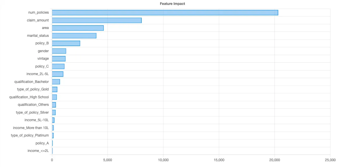
Computing Shapley values is computationally intensive and can take hours. We’ll use the Python SHAP library with some sampling to compute the following feature importance chart:

This tells us the major factors that are driving this particular computation.

What-If Analysis

We now know the number of policies is the biggest factor, followed by claim amount, followed by area. So, how exactly does the number of policies affect the average LTV?

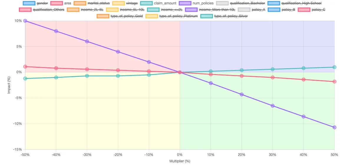
We can use our predictive model to answer this question. We take our original input data, and change the average number of policies up and down in 10% intervals. This lets us create a what-if chart like below, which shows the relative impact of changing the number of policies, area, and claim amounts.

• As the average number of policies increases, the average LTV decreases, as shown by the purple line. A 50% increase in policies causes a 10.7% decrease in average LTV.
• Claim amounts are represented by the teal line. As claim amounts increase, the average LTV modestly increases. A 50% increase in claim amount causes a 1% decrease in average LTV.
• Area is shown by the red line. Urban customers are slightly more valuable than rural customers. As the mix shifts towards urban by 50%, a 1.1% increase in average LTV is noted.

Next

Traditional models for LTV have historically focused on segmentation and aligning customer acquisition channels to specific segments. While effective, this approach often relies on predefined assumptions and can limit the scope of analysis. In contrast, regression analysis offers a powerful tool for at-scale data exploration, allowing for the analysis of possibilities that may not have been considered initially. Dashboards excel in the traditional model as they align with predefined questions, but regression analysis, especially when augmented with machine learning, can reveal insights that go beyond the scope of predefined queries. By embracing machine learning to enhance regression analysis, businesses can uncover new levers for customer acquisition and optimize their strategies for long-term success in a data-driven landscape.